> ## Documentation Index
> Fetch the complete documentation index at: https://nixtla-old-docs.mintlify.site/llms.txt
> Use this file to discover all available pages before exploring further.
> In this example we will show how to perform electricity load forecasting on the ERCOT (Texas) market for detecting daily peaks.
# Detect Demand Peaks
## Introduction
Predicting peaks in different markets is useful. In the electricity
market, consuming electricity at peak demand is penalized with higher
tarifs. When an individual or company consumes electricity when its most
demanded, regulators calls that a coincident peak (CP).
In the Texas electricity market (ERCOT), the peak is the monthly
15-minute interval when the ERCOT Grid is at a point of highest
capacity. The peak is caused by all consumers’ combined demand on the
electrical grid. The coincident peak demand is an important factor used
by ERCOT to determine final electricity consumption bills. ERCOT
registers the CP demand of each client for 4 months, between June and
September, and uses this to adjust electricity prices. Clients can
therefore save on electricity bills by reducing the coincident peak
demand.
In this example we will train an
[`MSTL`](../../src/core/models.html#mstl)
(Multiple Seasonal-Trend decomposition using LOESS) model on historic
load data to forecast day-ahead peaks on September 2022. Multiple
seasonality is traditionally present in low sampled electricity data.
Demand exhibits daily and weekly seasonality, with clear patterns for
specific hours of the day such as 6:00pm vs 3:00am or for specific days
such as Sunday vs Friday.
First, we will load ERCOT historic demand, then we will use the
[`StatsForecast.cross_validation`](../../src/core/core.html#statsforecast.cross_validation)
method to fit the MSTL model and forecast daily load during September.
Finally, we show how to use the forecasts to detect the coincident peak.
**Outline**
1. Install libraries
2. Load and explore the data
3. Fit MSTL model and forecast
4. Peak detection
> **Tip**
>
> You can use Colab to run this Notebook interactively
>
>
>  >
## Libraries
We assume you have StatsForecast already installed. Check this guide for
instructions on [how to install StatsForecast](../getting-started/installation.html).
Install the necessary packages using `pip install statsforecast`
## Load Data
The input to StatsForecast is always a data frame in [long
format](https://www.theanalysisfactor.com/wide-and-long-data/) with
three columns: `unique_id`, `ds` and `y`:
* The `unique_id` (string, int or category) represents an identifier
for the series.
* The `ds` (datestamp or int) column should be either an integer
indexing time or a datestamp ideally like YYYY-MM-DD for a date or
YYYY-MM-DD HH:MM:SS for a timestamp.
* The `y` (numeric) represents the measurement we wish to forecast.
```python theme={null}
import numpy as np
import pandas as pd
```
```python theme={null}
Y_df = pd.read_csv('https://datasets-nixtla.s3.amazonaws.com/ERCOT-clean.csv', parse_dates=['ds'])
```
Plot the series using the `plot` method from the
[`StatsForecast`](../../src/core/core.html#statsforecast-plot)
class. This method prints up to 8 random series from the dataset and is
useful for basic EDA.
> **Note**
>
> The `StatsForecast.plot` method uses Plotly as a default engine. You
> can change to MatPlotLib by setting `engine="matplotlib"`.
```python theme={null}
from statsforecast import StatsForecast
```
```python theme={null}
StatsForecast.plot(Y_df)
```
>
## Libraries
We assume you have StatsForecast already installed. Check this guide for
instructions on [how to install StatsForecast](../getting-started/installation.html).
Install the necessary packages using `pip install statsforecast`
## Load Data
The input to StatsForecast is always a data frame in [long
format](https://www.theanalysisfactor.com/wide-and-long-data/) with
three columns: `unique_id`, `ds` and `y`:
* The `unique_id` (string, int or category) represents an identifier
for the series.
* The `ds` (datestamp or int) column should be either an integer
indexing time or a datestamp ideally like YYYY-MM-DD for a date or
YYYY-MM-DD HH:MM:SS for a timestamp.
* The `y` (numeric) represents the measurement we wish to forecast.
```python theme={null}
import numpy as np
import pandas as pd
```
```python theme={null}
Y_df = pd.read_csv('https://datasets-nixtla.s3.amazonaws.com/ERCOT-clean.csv', parse_dates=['ds'])
```
Plot the series using the `plot` method from the
[`StatsForecast`](../../src/core/core.html#statsforecast-plot)
class. This method prints up to 8 random series from the dataset and is
useful for basic EDA.
> **Note**
>
> The `StatsForecast.plot` method uses Plotly as a default engine. You
> can change to MatPlotLib by setting `engine="matplotlib"`.
```python theme={null}
from statsforecast import StatsForecast
```
```python theme={null}
StatsForecast.plot(Y_df)
```
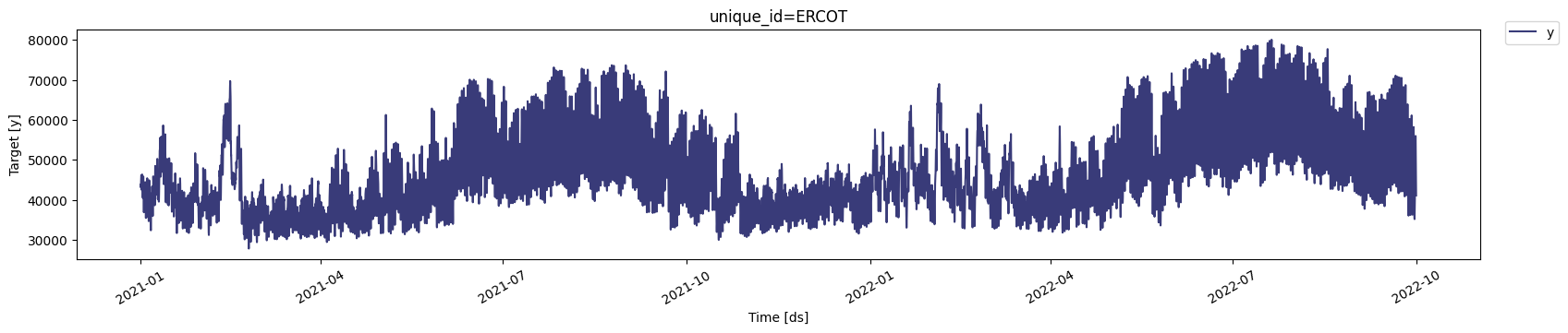 We observe that the time series exhibits seasonal patterns. Moreover,
the time series contains `6,552` observations, so it is necessary to use
computationally efficient methods to deploy them in production.
## Fit and Forecast MSTL model
The MSTL (Multiple Seasonal-Trend decomposition using LOESS) model
decomposes the time series in multiple seasonalities using a Local
Polynomial Regression (LOESS). Then it forecasts the trend using a
custom non-seasonal model and each seasonality using a SeasonalNaive
model.
> **Tip**
>
> Check our detailed explanation and tutorial on MSTL
> [here](./multipleseasonalities.html)
Import the
[`StatsForecast`](../../src/core/core.html#statsforecast)
class and the models you need.
```python theme={null}
from sklearn.linear_model import LinearRegression
from utilsforecast.feature_engineering import trend
from statsforecast import StatsForecast
from statsforecast.models import MSTL, SklearnModel
```
First, instantiate the model and define the parameters. The electricity
load presents seasonalities every 24 hours (Hourly) and every 24 \* 7
(Daily) hours. Therefore, we will use `[24, 24 * 7]` as the
seasonalities. See [this
link](https://robjhyndman.com/hyndsight/seasonal-periods/) for a
detailed explanation on how to set seasonal lengths. In this example we
use the
[`SklearnModel`](../../src/core/models.html#sklearnmodel)
with a `LinearRegression` model for the trend component, however, any
StatsForecast model can be used. The complete list of models is
available [here](../../src/core/models.html).
```python theme={null}
train, _ = trend(Y_df, freq='H')
train.head()
```
| | unique\_id | ds | y | trend |
| - | ---------- | ------------------- | ------------ | ----- |
| 0 | ERCOT | 2021-01-01 00:00:00 | 43719.849616 | 1.0 |
| 1 | ERCOT | 2021-01-01 01:00:00 | 43321.050347 | 2.0 |
| 2 | ERCOT | 2021-01-01 02:00:00 | 43063.067063 | 3.0 |
| 3 | ERCOT | 2021-01-01 03:00:00 | 43090.059203 | 4.0 |
| 4 | ERCOT | 2021-01-01 04:00:00 | 43486.590073 | 5.0 |
```python theme={null}
models = [
MSTL(
season_length=[24, 24 * 7], # seasonalities of the time series
trend_forecaster=SklearnModel(LinearRegression()) # model used to forecast trend
)
]
```
We fit the model by instantiating a
[`StatsForecast`](../../src/core/core.html#statsforecast)
object with the following required parameters:
* `models`: a list of models. Select the models you want from
[models](../models.html) and import them.
* `freq`: a string indicating the frequency of the data. (See [panda’s
available
frequencies](https://pandas.pydata.org/pandas-docs/stable/user_guide/timeseries.html#offset-aliases).)
```python theme={null}
# Instantiate StatsForecast class as sf
sf = StatsForecast(
models=models,
freq='H',
)
```
> **Tip**
>
> StatsForecast also supports this optional parameter.
>
> * `n_jobs`: n\_jobs: int, number of jobs used in the parallel
> processing, use -1 for all cores. (Default: 1)
>
> * `fallback_model`: a model to be used if a model fails. (Default:
> none)
The
[`cross_validation`](../../src/mfles.html#cross_validation)
method allows the user to simulate multiple historic forecasts, greatly
simplifying pipelines by replacing for loops with `fit` and `predict`
methods. This method re-trains the model and forecast each window. See
[this
tutorial](../getting-started/getting_started_complete.html)
for an animation of how the windows are defined.
Use the
[`cross_validation`](../../src/mfles.html#cross_validation)
method to produce all the daily forecasts for September. To produce
daily forecasts set the forecasting horizon `h` as 24. In this example
we are simulating deploying the pipeline during September, so set the
number of windows as 30 (one for each day). Finally, set the step size
between windows as 24, to only produce one forecast per day.
```python theme={null}
cv_df = sf.cross_validation(
df=train,
h=24,
step_size=24,
n_windows=30
)
```
```python theme={null}
cv_df.head()
```
| | unique\_id | ds | cutoff | y | MSTL |
| - | ---------- | ------------------- | ------------------- | ------------ | ------------ |
| 0 | ERCOT | 2022-09-01 00:00:00 | 2022-08-31 23:00:00 | 45482.471757 | 47413.944185 |
| 1 | ERCOT | 2022-09-01 01:00:00 | 2022-08-31 23:00:00 | 43602.658043 | 45237.153285 |
| 2 | ERCOT | 2022-09-01 02:00:00 | 2022-08-31 23:00:00 | 42284.817342 | 43816.390019 |
| 3 | ERCOT | 2022-09-01 03:00:00 | 2022-08-31 23:00:00 | 41663.156771 | 42972.956286 |
| 4 | ERCOT | 2022-09-01 04:00:00 | 2022-08-31 23:00:00 | 41710.621904 | 42909.899438 |
> **Important**
>
> When using
> [`cross_validation`](../../src/mfles.html#cross_validation)
> make sure the forecasts are produced at the desired timestamps. Check
> the `cutoff` column which specifices the last timestamp before the
> forecasting window.
## Peak Detection
Finally, we use the forecasts in `cv_df` to detect the daily hourly
demand peaks. For each day, we set the detected peaks as the highest
forecasts. In this case, we want to predict one peak (`npeaks`);
depending on your setting and goals, this parameter might change. For
example, the number of peaks can correspond to how many hours a battery
can be discharged to reduce demand.
```python theme={null}
npeaks = 1 # Number of peaks
```
For the ERCOT 4CP detection task we are interested in correctly
predicting the highest monthly load. Next, we filter the day in
September with the highest hourly demand and predict the peak.
```python theme={null}
cv_df = cv_df[['ds','y','MSTL']]
max_day = cv_df.iloc[cv_df['y'].argmax()].ds.day # Day with maximum load
cv_df_day = cv_df.query('ds.dt.day == @max_day')
max_hour = cv_df_day['y'].argmax()
peaks = cv_df_day['MSTL'].argsort().iloc[-npeaks:].values # Predicted peaks
```
In the following plot we see how the MSTL model is able to correctly
detect the coincident peak for September 2022.
```python theme={null}
import matplotlib.pyplot as plt
```
```python theme={null}
plt.figure(figsize=(10, 5))
plt.axvline(cv_df_day.iloc[max_hour]['ds'], color='black', label='True Peak')
plt.scatter(cv_df_day.iloc[peaks]['ds'], cv_df_day.iloc[peaks]['MSTL'], color='green', label=f'Predicted Top-{npeaks}')
plt.plot(cv_df_day['ds'], cv_df_day['y'], label='y', color='blue')
plt.plot(cv_df_day['ds'], cv_df_day['MSTL'], label='Forecast', color='red')
plt.xlabel('Time')
plt.ylabel('Load (MW)')
plt.grid()
plt.legend()
```
We observe that the time series exhibits seasonal patterns. Moreover,
the time series contains `6,552` observations, so it is necessary to use
computationally efficient methods to deploy them in production.
## Fit and Forecast MSTL model
The MSTL (Multiple Seasonal-Trend decomposition using LOESS) model
decomposes the time series in multiple seasonalities using a Local
Polynomial Regression (LOESS). Then it forecasts the trend using a
custom non-seasonal model and each seasonality using a SeasonalNaive
model.
> **Tip**
>
> Check our detailed explanation and tutorial on MSTL
> [here](./multipleseasonalities.html)
Import the
[`StatsForecast`](../../src/core/core.html#statsforecast)
class and the models you need.
```python theme={null}
from sklearn.linear_model import LinearRegression
from utilsforecast.feature_engineering import trend
from statsforecast import StatsForecast
from statsforecast.models import MSTL, SklearnModel
```
First, instantiate the model and define the parameters. The electricity
load presents seasonalities every 24 hours (Hourly) and every 24 \* 7
(Daily) hours. Therefore, we will use `[24, 24 * 7]` as the
seasonalities. See [this
link](https://robjhyndman.com/hyndsight/seasonal-periods/) for a
detailed explanation on how to set seasonal lengths. In this example we
use the
[`SklearnModel`](../../src/core/models.html#sklearnmodel)
with a `LinearRegression` model for the trend component, however, any
StatsForecast model can be used. The complete list of models is
available [here](../../src/core/models.html).
```python theme={null}
train, _ = trend(Y_df, freq='H')
train.head()
```
| | unique\_id | ds | y | trend |
| - | ---------- | ------------------- | ------------ | ----- |
| 0 | ERCOT | 2021-01-01 00:00:00 | 43719.849616 | 1.0 |
| 1 | ERCOT | 2021-01-01 01:00:00 | 43321.050347 | 2.0 |
| 2 | ERCOT | 2021-01-01 02:00:00 | 43063.067063 | 3.0 |
| 3 | ERCOT | 2021-01-01 03:00:00 | 43090.059203 | 4.0 |
| 4 | ERCOT | 2021-01-01 04:00:00 | 43486.590073 | 5.0 |
```python theme={null}
models = [
MSTL(
season_length=[24, 24 * 7], # seasonalities of the time series
trend_forecaster=SklearnModel(LinearRegression()) # model used to forecast trend
)
]
```
We fit the model by instantiating a
[`StatsForecast`](../../src/core/core.html#statsforecast)
object with the following required parameters:
* `models`: a list of models. Select the models you want from
[models](../models.html) and import them.
* `freq`: a string indicating the frequency of the data. (See [panda’s
available
frequencies](https://pandas.pydata.org/pandas-docs/stable/user_guide/timeseries.html#offset-aliases).)
```python theme={null}
# Instantiate StatsForecast class as sf
sf = StatsForecast(
models=models,
freq='H',
)
```
> **Tip**
>
> StatsForecast also supports this optional parameter.
>
> * `n_jobs`: n\_jobs: int, number of jobs used in the parallel
> processing, use -1 for all cores. (Default: 1)
>
> * `fallback_model`: a model to be used if a model fails. (Default:
> none)
The
[`cross_validation`](../../src/mfles.html#cross_validation)
method allows the user to simulate multiple historic forecasts, greatly
simplifying pipelines by replacing for loops with `fit` and `predict`
methods. This method re-trains the model and forecast each window. See
[this
tutorial](../getting-started/getting_started_complete.html)
for an animation of how the windows are defined.
Use the
[`cross_validation`](../../src/mfles.html#cross_validation)
method to produce all the daily forecasts for September. To produce
daily forecasts set the forecasting horizon `h` as 24. In this example
we are simulating deploying the pipeline during September, so set the
number of windows as 30 (one for each day). Finally, set the step size
between windows as 24, to only produce one forecast per day.
```python theme={null}
cv_df = sf.cross_validation(
df=train,
h=24,
step_size=24,
n_windows=30
)
```
```python theme={null}
cv_df.head()
```
| | unique\_id | ds | cutoff | y | MSTL |
| - | ---------- | ------------------- | ------------------- | ------------ | ------------ |
| 0 | ERCOT | 2022-09-01 00:00:00 | 2022-08-31 23:00:00 | 45482.471757 | 47413.944185 |
| 1 | ERCOT | 2022-09-01 01:00:00 | 2022-08-31 23:00:00 | 43602.658043 | 45237.153285 |
| 2 | ERCOT | 2022-09-01 02:00:00 | 2022-08-31 23:00:00 | 42284.817342 | 43816.390019 |
| 3 | ERCOT | 2022-09-01 03:00:00 | 2022-08-31 23:00:00 | 41663.156771 | 42972.956286 |
| 4 | ERCOT | 2022-09-01 04:00:00 | 2022-08-31 23:00:00 | 41710.621904 | 42909.899438 |
> **Important**
>
> When using
> [`cross_validation`](../../src/mfles.html#cross_validation)
> make sure the forecasts are produced at the desired timestamps. Check
> the `cutoff` column which specifices the last timestamp before the
> forecasting window.
## Peak Detection
Finally, we use the forecasts in `cv_df` to detect the daily hourly
demand peaks. For each day, we set the detected peaks as the highest
forecasts. In this case, we want to predict one peak (`npeaks`);
depending on your setting and goals, this parameter might change. For
example, the number of peaks can correspond to how many hours a battery
can be discharged to reduce demand.
```python theme={null}
npeaks = 1 # Number of peaks
```
For the ERCOT 4CP detection task we are interested in correctly
predicting the highest monthly load. Next, we filter the day in
September with the highest hourly demand and predict the peak.
```python theme={null}
cv_df = cv_df[['ds','y','MSTL']]
max_day = cv_df.iloc[cv_df['y'].argmax()].ds.day # Day with maximum load
cv_df_day = cv_df.query('ds.dt.day == @max_day')
max_hour = cv_df_day['y'].argmax()
peaks = cv_df_day['MSTL'].argsort().iloc[-npeaks:].values # Predicted peaks
```
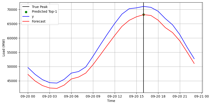
In the following plot we see how the MSTL model is able to correctly
detect the coincident peak for September 2022.
```python theme={null}
import matplotlib.pyplot as plt
```
```python theme={null}
plt.figure(figsize=(10, 5))
plt.axvline(cv_df_day.iloc[max_hour]['ds'], color='black', label='True Peak')
plt.scatter(cv_df_day.iloc[peaks]['ds'], cv_df_day.iloc[peaks]['MSTL'], color='green', label=f'Predicted Top-{npeaks}')
plt.plot(cv_df_day['ds'], cv_df_day['y'], label='y', color='blue')
plt.plot(cv_df_day['ds'], cv_df_day['MSTL'], label='Forecast', color='red')
plt.xlabel('Time')
plt.ylabel('Load (MW)')
plt.grid()
plt.legend()
```
 > **Important**
>
> In this example we only include September. However, MSTL can correctly
> predict the peaks for the 4 months of 2022. You can try this by
> increasing the `nwindows` parameter of
> [`cross_validation`](../../src/mfles.html#cross_validation)
> or filtering the `Y_df` dataset. The complete run for all months take
> only 10 minutes.
## Next steps
StatsForecast and MSTL in particular are good benchmarking models for
peak detection. However, it might be useful to explore further and newer
forecasting algorithms. We have seen particularly good results with the
N-HiTS, a deep-learning model from Nixtla’s NeuralForecast library.
Learn how to predict ERCOT demand peaks with our deep-learning N-HiTS
model and the NeuralForecast library in [this
tutorial](../../../neuralforecast/docs/use-cases/electricity_peak_forecasting.html).
## References
* [Bandara, Kasun & Hyndman, Rob & Bergmeir, Christoph. (2021). “MSTL:
A Seasonal-Trend Decomposition Algorithm for Time Series with
Multiple Seasonal Patterns”](https://arxiv.org/abs/2107.13462).
* [Cristian Challu, Kin G. Olivares, Boris N. Oreshkin, Federico
Garza, Max Mergenthaler-Canseco, Artur Dubrawski (2021). “N-HiTS:
Neural Hierarchical Interpolation for Time Series Forecasting”.
Accepted at AAAI 2023.](https://arxiv.org/abs/2201.12886)
> **Important**
>
> In this example we only include September. However, MSTL can correctly
> predict the peaks for the 4 months of 2022. You can try this by
> increasing the `nwindows` parameter of
> [`cross_validation`](../../src/mfles.html#cross_validation)
> or filtering the `Y_df` dataset. The complete run for all months take
> only 10 minutes.
## Next steps
StatsForecast and MSTL in particular are good benchmarking models for
peak detection. However, it might be useful to explore further and newer
forecasting algorithms. We have seen particularly good results with the
N-HiTS, a deep-learning model from Nixtla’s NeuralForecast library.
Learn how to predict ERCOT demand peaks with our deep-learning N-HiTS
model and the NeuralForecast library in [this
tutorial](../../../neuralforecast/docs/use-cases/electricity_peak_forecasting.html).
## References
* [Bandara, Kasun & Hyndman, Rob & Bergmeir, Christoph. (2021). “MSTL:
A Seasonal-Trend Decomposition Algorithm for Time Series with
Multiple Seasonal Patterns”](https://arxiv.org/abs/2107.13462).
* [Cristian Challu, Kin G. Olivares, Boris N. Oreshkin, Federico
Garza, Max Mergenthaler-Canseco, Artur Dubrawski (2021). “N-HiTS:
Neural Hierarchical Interpolation for Time Series Forecasting”.
Accepted at AAAI 2023.](https://arxiv.org/abs/2201.12886)