> ## Documentation Index
> Fetch the complete documentation index at: https://nixtla-old-docs.mintlify.site/llms.txt
> Use this file to discover all available pages before exploring further.
> NeuralForecast contains a collection NumPy loss functions aimed to be used during the models' evaluation.
# NumPy Evaluation
The most important train signal is the forecast error, which is the
difference between the observed value $y_{\tau}$ and the prediction
$\hat{y}_{\tau}$, at time $y_{\tau}$:
$e_{\tau} = y_{\tau}-\hat{y}_{\tau} \qquad \qquad \tau \in \{t+1,\dots,t+H \}$
The train loss summarizes the forecast errors in different evaluation
metrics.
# 1. Scale-dependent Errors
These metrics are on the same scale as the data.
## Mean Absolute Error
***
source
### mae
> ```text theme={null}
> mae (y:numpy.ndarray, y_hat:numpy.ndarray,
> weights:Optional[numpy.ndarray]=None, axis:Optional[int]=None)
> ```
\*Mean Absolute Error
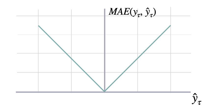
Calculates Mean Absolute Error between `y` and `y_hat`. MAE measures the
relative prediction accuracy of a forecasting method by calculating the
deviation of the prediction and the true value at a given time and
averages these devations over the length of the series.
$\mathrm{MAE}(\mathbf{y}_{\tau}, \mathbf{\hat{y}}_{\tau}) = \frac{1}{H} \sum^{t+H}_{\tau=t+1} |y_{\tau} - \hat{y}_{\tau}|$
**Parameters:**
`y`: numpy array, Actual values.
`y_hat`: numpy
array, Predicted values.
`mask`: numpy array, Specifies date stamps
per serie to consider in loss.
**Returns:**
[`mae`](https://nixtlaverse.nixtla.io/neuralforecast/losses.numpy.html#mae):
numpy array, (single value).\*
 ## Mean Squared Error
***
source
### mse
> ```text theme={null}
> mse (y:numpy.ndarray, y_hat:numpy.ndarray,
> weights:Optional[numpy.ndarray]=None, axis:Optional[int]=None)
> ```
\*Mean Squared Error
Calculates Mean Squared Error between `y` and `y_hat`. MSE measures the
relative prediction accuracy of a forecasting method by calculating the
squared deviation of the prediction and the true value at a given time,
and averages these devations over the length of the series.
$\mathrm{MSE}(\mathbf{y}_{\tau}, \mathbf{\hat{y}}_{\tau}) = \frac{1}{H} \sum^{t+H}_{\tau=t+1} (y_{\tau} - \hat{y}_{\tau})^{2}$
**Parameters:**
## Mean Squared Error
***
source
### mse
> ```text theme={null}
> mse (y:numpy.ndarray, y_hat:numpy.ndarray,
> weights:Optional[numpy.ndarray]=None, axis:Optional[int]=None)
> ```
\*Mean Squared Error
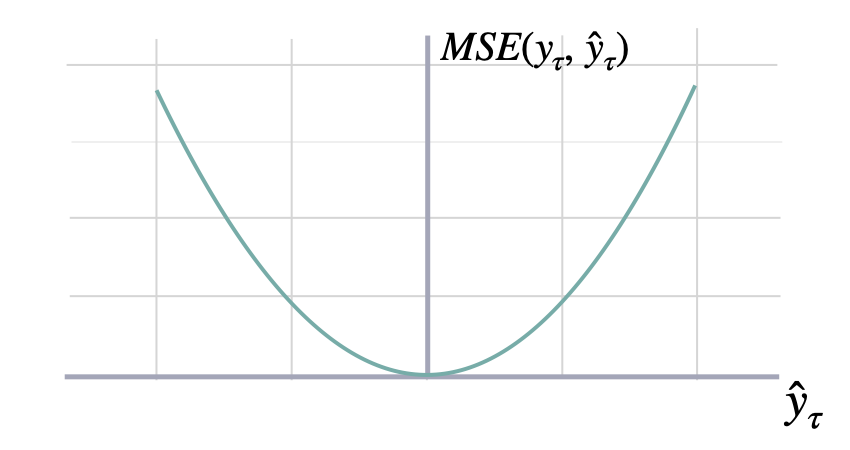
Calculates Mean Squared Error between `y` and `y_hat`. MSE measures the
relative prediction accuracy of a forecasting method by calculating the
squared deviation of the prediction and the true value at a given time,
and averages these devations over the length of the series.
$\mathrm{MSE}(\mathbf{y}_{\tau}, \mathbf{\hat{y}}_{\tau}) = \frac{1}{H} \sum^{t+H}_{\tau=t+1} (y_{\tau} - \hat{y}_{\tau})^{2}$
**Parameters:**
`y`: numpy array, Actual values.
`y_hat`: numpy
array, Predicted values.
`mask`: numpy array, Specifies date stamps
per serie to consider in loss.
**Returns:**
[`mse`](https://nixtlaverse.nixtla.io/neuralforecast/losses.numpy.html#mse):
numpy array, (single value).\*
 ## Root Mean Squared Error
***
source
### rmse
> ```text theme={null}
> rmse (y:numpy.ndarray, y_hat:numpy.ndarray,
> weights:Optional[numpy.ndarray]=None, axis:Optional[int]=None)
> ```
\*Root Mean Squared Error
Calculates Root Mean Squared Error between `y` and `y_hat`. RMSE
measures the relative prediction accuracy of a forecasting method by
calculating the squared deviation of the prediction and the observed
value at a given time and averages these devations over the length of
the series. Finally the RMSE will be in the same scale as the original
time series so its comparison with other series is possible only if they
share a common scale. RMSE has a direct connection to the L2 norm.
$\mathrm{RMSE}(\mathbf{y}_{\tau}, \mathbf{\hat{y}}_{\tau}) = \sqrt{\frac{1}{H} \sum^{t+H}_{\tau=t+1} (y_{\tau} - \hat{y}_{\tau})^{2}}$
**Parameters:**
## Root Mean Squared Error
***
source
### rmse
> ```text theme={null}
> rmse (y:numpy.ndarray, y_hat:numpy.ndarray,
> weights:Optional[numpy.ndarray]=None, axis:Optional[int]=None)
> ```
\*Root Mean Squared Error
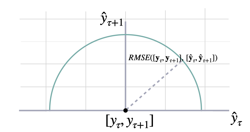
Calculates Root Mean Squared Error between `y` and `y_hat`. RMSE
measures the relative prediction accuracy of a forecasting method by
calculating the squared deviation of the prediction and the observed
value at a given time and averages these devations over the length of
the series. Finally the RMSE will be in the same scale as the original
time series so its comparison with other series is possible only if they
share a common scale. RMSE has a direct connection to the L2 norm.
$\mathrm{RMSE}(\mathbf{y}_{\tau}, \mathbf{\hat{y}}_{\tau}) = \sqrt{\frac{1}{H} \sum^{t+H}_{\tau=t+1} (y_{\tau} - \hat{y}_{\tau})^{2}}$
**Parameters:**
`y`: numpy array, Actual values.
`y_hat`: numpy
array, Predicted values.
`mask`: numpy array, Specifies date stamps
per serie to consider in loss.
**Returns:**
[`rmse`](https://nixtlaverse.nixtla.io/neuralforecast/losses.numpy.html#rmse):
numpy array, (single value).\*
 # 2. Percentage errors
These metrics are unit-free, suitable for comparisons across series.
## Mean Absolute Percentage Error
***
source
### mape
> ```text theme={null}
> mape (y:numpy.ndarray, y_hat:numpy.ndarray,
> weights:Optional[numpy.ndarray]=None, axis:Optional[int]=None)
> ```
\*Mean Absolute Percentage Error
Calculates Mean Absolute Percentage Error between `y` and `y_hat`. MAPE
measures the relative prediction accuracy of a forecasting method by
calculating the percentual deviation of the prediction and the observed
value at a given time and averages these devations over the length of
the series. The closer to zero an observed value is, the higher penalty
MAPE loss assigns to the corresponding error.
$\mathrm{MAPE}(\mathbf{y}_{\tau}, \mathbf{\hat{y}}_{\tau}) = \frac{1}{H} \sum^{t+H}_{\tau=t+1} \frac{|y_{\tau}-\hat{y}_{\tau}|}{|y_{\tau}|}$
**Parameters:**
# 2. Percentage errors
These metrics are unit-free, suitable for comparisons across series.
## Mean Absolute Percentage Error
***
source
### mape
> ```text theme={null}
> mape (y:numpy.ndarray, y_hat:numpy.ndarray,
> weights:Optional[numpy.ndarray]=None, axis:Optional[int]=None)
> ```
\*Mean Absolute Percentage Error
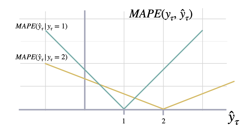
Calculates Mean Absolute Percentage Error between `y` and `y_hat`. MAPE
measures the relative prediction accuracy of a forecasting method by
calculating the percentual deviation of the prediction and the observed
value at a given time and averages these devations over the length of
the series. The closer to zero an observed value is, the higher penalty
MAPE loss assigns to the corresponding error.
$\mathrm{MAPE}(\mathbf{y}_{\tau}, \mathbf{\hat{y}}_{\tau}) = \frac{1}{H} \sum^{t+H}_{\tau=t+1} \frac{|y_{\tau}-\hat{y}_{\tau}|}{|y_{\tau}|}$
**Parameters:**
`y`: numpy array, Actual values.
`y_hat`: numpy
array, Predicted values.
`mask`: numpy array, Specifies date stamps
per serie to consider in loss.
**Returns:**
[`mape`](https://nixtlaverse.nixtla.io/neuralforecast/losses.numpy.html#mape):
numpy array, (single value).\*
 ## SMAPE
***
source
### smape
> ```text theme={null}
> smape (y:numpy.ndarray, y_hat:numpy.ndarray,
> weights:Optional[numpy.ndarray]=None, axis:Optional[int]=None)
> ```
\*Symmetric Mean Absolute Percentage Error
Calculates Symmetric Mean Absolute Percentage Error between `y` and
`y_hat`. SMAPE measures the relative prediction accuracy of a
forecasting method by calculating the relative deviation of the
prediction and the observed value scaled by the sum of the absolute
values for the prediction and observed value at a given time, then
averages these devations over the length of the series. This allows the
SMAPE to have bounds between 0% and 200% which is desirable compared to
normal MAPE that may be undetermined when the target is zero.
$\mathrm{sMAPE}_{2}(\mathbf{y}_{\tau}, \mathbf{\hat{y}}_{\tau}) = \frac{1}{H} \sum^{t+H}_{\tau=t+1} \frac{|y_{\tau}-\hat{y}_{\tau}|}{|y_{\tau}|+|\hat{y}_{\tau}|}$
**Parameters:**
## SMAPE
***
source
### smape
> ```text theme={null}
> smape (y:numpy.ndarray, y_hat:numpy.ndarray,
> weights:Optional[numpy.ndarray]=None, axis:Optional[int]=None)
> ```
\*Symmetric Mean Absolute Percentage Error
Calculates Symmetric Mean Absolute Percentage Error between `y` and
`y_hat`. SMAPE measures the relative prediction accuracy of a
forecasting method by calculating the relative deviation of the
prediction and the observed value scaled by the sum of the absolute
values for the prediction and observed value at a given time, then
averages these devations over the length of the series. This allows the
SMAPE to have bounds between 0% and 200% which is desirable compared to
normal MAPE that may be undetermined when the target is zero.
$\mathrm{sMAPE}_{2}(\mathbf{y}_{\tau}, \mathbf{\hat{y}}_{\tau}) = \frac{1}{H} \sum^{t+H}_{\tau=t+1} \frac{|y_{\tau}-\hat{y}_{\tau}|}{|y_{\tau}|+|\hat{y}_{\tau}|}$
**Parameters:**
`y`: numpy array, Actual values.
`y_hat`: numpy
array, Predicted values.
`mask`: numpy array, Specifies date stamps
per serie to consider in loss.
**Returns:**
[`smape`](https://nixtlaverse.nixtla.io/neuralforecast/losses.numpy.html#smape):
numpy array, (single value).
**References:**
[Makridakis S., “Accuracy measures: theoretical and
practical
concerns”.](https://www.sciencedirect.com/science/article/pii/0169207093900793)\*
# 3. Scale-independent Errors
These metrics measure the relative improvements versus baselines.
## Mean Absolute Scaled Error
***
source
### mase
> ```text theme={null}
> mase (y:numpy.ndarray, y_hat:numpy.ndarray, y_train:numpy.ndarray,
> seasonality:int, weights:Optional[numpy.ndarray]=None,
> axis:Optional[int]=None)
> ```
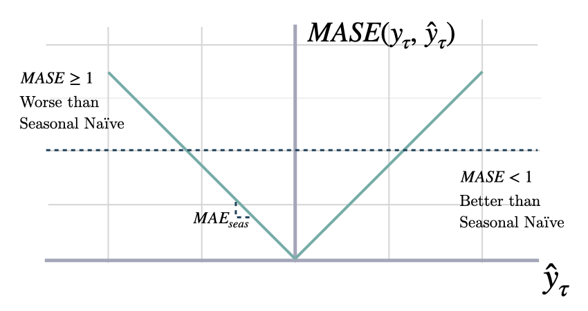
\*Mean Absolute Scaled Error Calculates the Mean Absolute Scaled Error
between `y` and `y_hat`. MASE measures the relative prediction accuracy
of a forecasting method by comparinng the mean absolute errors of the
prediction and the observed value against the mean absolute errors of
the seasonal naive model. The MASE partially composed the Overall
Weighted Average (OWA), used in the M4 Competition.
$\mathrm{MASE}(\mathbf{y}_{\tau}, \mathbf{\hat{y}}_{\tau}, \mathbf{\hat{y}}^{season}_{\tau}) = \frac{1}{H} \sum^{t+H}_{\tau=t+1} \frac{|y_{\tau}-\hat{y}_{\tau}|}{\mathrm{MAE}(\mathbf{y}_{\tau}, \mathbf{\hat{y}}^{season}_{\tau})}$
**Parameters:**
`y`: numpy array, (batch\_size, output\_size), Actual
values.
`y_hat`: numpy array, (batch\_size, output\_size)), Predicted
values.
`y_insample`: numpy array, (batch\_size, input\_size), Actual
insample Seasonal Naive predictions.
`seasonality`: int. Main
frequency of the time series; Hourly 24, Daily 7, Weekly 52, Monthly 12,
Quarterly 4, Yearly 1.\
`mask`: numpy array, Specifies date stamps per serie to consider in
loss.
**Returns:**
[`mase`](https://nixtlaverse.nixtla.io/neuralforecast/losses.numpy.html#mase):
numpy array, (single value).
**References:**
[Rob J. Hyndman, & Koehler, A. B. “Another look at
measures of forecast
accuracy”.](https://www.sciencedirect.com/science/article/pii/S0169207006000239)
[Spyros Makridakis, Evangelos Spiliotis, Vassilios Assimakopoulos, “The
M4 Competition: 100,000 time series and 61 forecasting
methods”.](https://www.sciencedirect.com/science/article/pii/S0169207019301128)\*
 ## Relative Mean Absolute Error
***
source
### rmae
> ```text theme={null}
> rmae (y:numpy.ndarray, y_hat1:numpy.ndarray, y_hat2:numpy.ndarray,
> weights:Optional[numpy.ndarray]=None, axis:Optional[int]=None)
> ```
\*RMAE
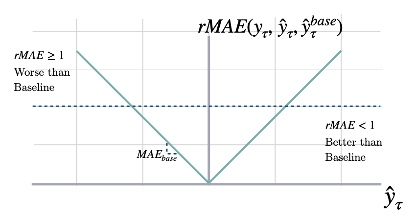
Calculates Relative Mean Absolute Error (RMAE) between two sets of
forecasts (from two different forecasting methods). A number smaller
than one implies that the forecast in the numerator is better than the
forecast in the denominator.
$\mathrm{rMAE}(\mathbf{y}_{\tau}, \mathbf{\hat{y}}_{\tau}, \mathbf{\hat{y}}^{base}_{\tau}) = \frac{1}{H} \sum^{t+H}_{\tau=t+1} \frac{|y_{\tau}-\hat{y}_{\tau}|}{\mathrm{MAE}(\mathbf{y}_{\tau}, \mathbf{\hat{y}}^{base}_{\tau})}$
**Parameters:**
## Relative Mean Absolute Error
***
source
### rmae
> ```text theme={null}
> rmae (y:numpy.ndarray, y_hat1:numpy.ndarray, y_hat2:numpy.ndarray,
> weights:Optional[numpy.ndarray]=None, axis:Optional[int]=None)
> ```
\*RMAE
Calculates Relative Mean Absolute Error (RMAE) between two sets of
forecasts (from two different forecasting methods). A number smaller
than one implies that the forecast in the numerator is better than the
forecast in the denominator.
$\mathrm{rMAE}(\mathbf{y}_{\tau}, \mathbf{\hat{y}}_{\tau}, \mathbf{\hat{y}}^{base}_{\tau}) = \frac{1}{H} \sum^{t+H}_{\tau=t+1} \frac{|y_{\tau}-\hat{y}_{\tau}|}{\mathrm{MAE}(\mathbf{y}_{\tau}, \mathbf{\hat{y}}^{base}_{\tau})}$
**Parameters:**
`y`: numpy array, observed values.
`y_hat1`:
numpy array. Predicted values of first model.
`y_hat2`: numpy array.
Predicted values of baseline model.
`weights`: numpy array,
optional. Weights for weighted average.
`axis`: None or int,
optional.Axis or axes along which to average a.
The default,
axis=None, will average over all of the elements of the input array.
**Returns:**
[`rmae`](https://nixtlaverse.nixtla.io/neuralforecast/losses.numpy.html#rmae):
numpy array or double.
**References:**
[Rob J. Hyndman, & Koehler, A. B. “Another look at
measures of forecast
accuracy”.](https://www.sciencedirect.com/science/article/pii/S0169207006000239)\*
 # 4. Probabilistic Errors
These measure absolute deviation non-symmetrically, that produce
under/over estimation.
## Quantile Loss
***
source
### quantile\_loss
> ```text theme={null}
> quantile_loss (y:numpy.ndarray, y_hat:numpy.ndarray, q:float=0.5,
> weights:Optional[numpy.ndarray]=None,
> axis:Optional[int]=None)
> ```
\*Quantile Loss
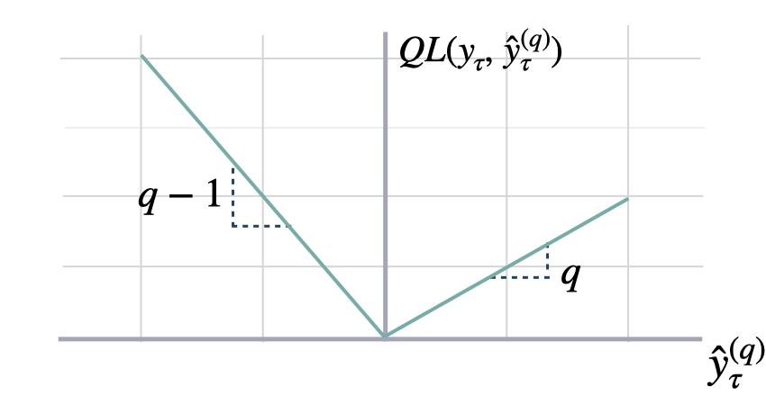
Computes the quantile loss between `y` and `y_hat`. QL measures the
deviation of a quantile forecast. By weighting the absolute deviation in
a non symmetric way, the loss pays more attention to under or over
estimation. A common value for q is 0.5 for the deviation from the
median (Pinball loss).
$\mathrm{QL}(\mathbf{y}_{\tau}, \mathbf{\hat{y}}^{(q)}_{\tau}) = \frac{1}{H} \sum^{t+H}_{\tau=t+1} \Big( (1-q)\,( \hat{y}^{(q)}_{\tau} - y_{\tau} )_{+} + q\,( y_{\tau} - \hat{y}^{(q)}_{\tau} )_{+} \Big)$
**Parameters:**
# 4. Probabilistic Errors
These measure absolute deviation non-symmetrically, that produce
under/over estimation.
## Quantile Loss
***
source
### quantile\_loss
> ```text theme={null}
> quantile_loss (y:numpy.ndarray, y_hat:numpy.ndarray, q:float=0.5,
> weights:Optional[numpy.ndarray]=None,
> axis:Optional[int]=None)
> ```
\*Quantile Loss
Computes the quantile loss between `y` and `y_hat`. QL measures the
deviation of a quantile forecast. By weighting the absolute deviation in
a non symmetric way, the loss pays more attention to under or over
estimation. A common value for q is 0.5 for the deviation from the
median (Pinball loss).
$\mathrm{QL}(\mathbf{y}_{\tau}, \mathbf{\hat{y}}^{(q)}_{\tau}) = \frac{1}{H} \sum^{t+H}_{\tau=t+1} \Big( (1-q)\,( \hat{y}^{(q)}_{\tau} - y_{\tau} )_{+} + q\,( y_{\tau} - \hat{y}^{(q)}_{\tau} )_{+} \Big)$
**Parameters:**
`y`: numpy array, Actual values.
`y_hat`: numpy
array, Predicted values.
`q`: float, between 0 and 1. The slope of
the quantile loss, in the context of quantile regression, the q
determines the conditional quantile level.
`mask`: numpy array,
Specifies date stamps per serie to consider in loss.
**Returns:**
[`quantile_loss`](https://nixtlaverse.nixtla.io/neuralforecast/losses.numpy.html#quantile_loss):
numpy array, (single value).
**References:**
[Roger Koenker and Gilbert Bassett, Jr., “Regression
Quantiles”.](https://www.jstor.org/stable/1913643)\*
 ## Multi-Quantile Loss
***
source
### mqloss
> ```text theme={null}
> mqloss (y:numpy.ndarray, y_hat:numpy.ndarray, quantiles:numpy.ndarray,
> weights:Optional[numpy.ndarray]=None, axis:Optional[int]=None)
> ```
\*Multi-Quantile loss
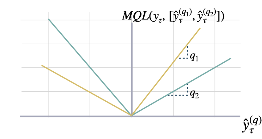
Calculates the Multi-Quantile loss (MQL) between `y` and `y_hat`. MQL
calculates the average multi-quantile Loss for a given set of quantiles,
based on the absolute difference between predicted quantiles and
observed values.
$\mathrm{MQL}(\mathbf{y}_{\tau},[\mathbf{\hat{y}}^{(q_{1})}_{\tau}, ... ,\hat{y}^{(q_{n})}_{\tau}]) = \frac{1}{n} \sum_{q_{i}} \mathrm{QL}(\mathbf{y}_{\tau}, \mathbf{\hat{y}}^{(q_{i})}_{\tau})$
The limit behavior of MQL allows to measure the accuracy of a full
predictive distribution $\mathbf{\hat{F}}_{\tau}$ with the continuous
ranked probability score (CRPS). This can be achieved through a
numerical integration technique, that discretizes the quantiles and
treats the CRPS integral with a left Riemann approximation, averaging
over uniformly distanced quantiles.
$\mathrm{CRPS}(y_{\tau}, \mathbf{\hat{F}}_{\tau}) = \int^{1}_{0} \mathrm{QL}(y_{\tau}, \hat{y}^{(q)}_{\tau}) dq$
**Parameters:**
## Multi-Quantile Loss
***
source
### mqloss
> ```text theme={null}
> mqloss (y:numpy.ndarray, y_hat:numpy.ndarray, quantiles:numpy.ndarray,
> weights:Optional[numpy.ndarray]=None, axis:Optional[int]=None)
> ```
\*Multi-Quantile loss
Calculates the Multi-Quantile loss (MQL) between `y` and `y_hat`. MQL
calculates the average multi-quantile Loss for a given set of quantiles,
based on the absolute difference between predicted quantiles and
observed values.
$\mathrm{MQL}(\mathbf{y}_{\tau},[\mathbf{\hat{y}}^{(q_{1})}_{\tau}, ... ,\hat{y}^{(q_{n})}_{\tau}]) = \frac{1}{n} \sum_{q_{i}} \mathrm{QL}(\mathbf{y}_{\tau}, \mathbf{\hat{y}}^{(q_{i})}_{\tau})$
The limit behavior of MQL allows to measure the accuracy of a full
predictive distribution $\mathbf{\hat{F}}_{\tau}$ with the continuous
ranked probability score (CRPS). This can be achieved through a
numerical integration technique, that discretizes the quantiles and
treats the CRPS integral with a left Riemann approximation, averaging
over uniformly distanced quantiles.
$\mathrm{CRPS}(y_{\tau}, \mathbf{\hat{F}}_{\tau}) = \int^{1}_{0} \mathrm{QL}(y_{\tau}, \hat{y}^{(q)}_{\tau}) dq$
**Parameters:**
`y`: numpy array, Actual values.
`y_hat`: numpy
array, Predicted values.
`quantiles`: numpy array,(n\_quantiles).
Quantiles to estimate from the distribution of y.
`mask`: numpy
array, Specifies date stamps per serie to consider in loss.
**Returns:**
[`mqloss`](https://nixtlaverse.nixtla.io/neuralforecast/losses.numpy.html#mqloss):
numpy array, (single value).
**References:**
[Roger Koenker and Gilbert Bassett, Jr., “Regression
Quantiles”.](https://www.jstor.org/stable/1913643)
[James E.
Matheson and Robert L. Winkler, “Scoring Rules for Continuous
Probability Distributions”.](https://www.jstor.org/stable/2629907)\*
 # Examples and Validation
```python theme={null}
import unittest
import torch as t
import numpy as np
from neuralforecast.losses.pytorch import (
MAE, MSE, RMSE, # unscaled errors
MAPE, SMAPE, # percentage errors
MASE, # scaled error
QuantileLoss, MQLoss # probabilistic errors
)
from neuralforecast.losses.numpy import (
mae, mse, rmse, # unscaled errors
mape, smape, # percentage errors
mase, # scaled error
quantile_loss, mqloss # probabilistic errors
)
```
# Examples and Validation
```python theme={null}
import unittest
import torch as t
import numpy as np
from neuralforecast.losses.pytorch import (
MAE, MSE, RMSE, # unscaled errors
MAPE, SMAPE, # percentage errors
MASE, # scaled error
QuantileLoss, MQLoss # probabilistic errors
)
from neuralforecast.losses.numpy import (
mae, mse, rmse, # unscaled errors
mape, smape, # percentage errors
mase, # scaled error
quantile_loss, mqloss # probabilistic errors
)
```